
The first milestone of Beyond 5s introduced a temporal B+ tree for FoundationDB’s conflict history under a memory budget. Packing many entries into each node improves locality and amortizes structural overhead. Variable-length key bytes are packed separately into linked blocks, keeping nodes compact. Point ranges [k, k\0) share their endpoint bytes: for a key of length L, they store L + 1 bytes instead of 2L + 1, nearly halving the key payload.
V1 also introduced proactive split preparation. Internal nodes reserve room for children that will need splitting, so each write splits at most one existing node. This distributes structural work across writes and removes cascading splits as a source of insertion-latency spikes.
Under 6 GiB, v1 retained 2.2× the history of the original skip list and made the same conflict decisions. It also took 2.7× as long to resolve the same trace, with reads accounting for the larger part of that gap.
V1 checked each read independently: a descent from the root, a search inside the leaf, a predecessor lookup, and a forward scan. Separator comparisons accessed key bytes stored outside the nodes. These dependent accesses were processed one read at a time, leaving an opportunity to share search work and overlap memory latency across reads.
Resolver v2 keeps v1’s representation, write path and reclamation model and rebuilds the read check around three ideas. The resolver already sorts a batch’s range endpoints, so the tree can extract the read begins in order and route them together by recursive partitioning, with far fewer comparisons than one descent per read. Reads that land in the same leaf are then checked as a group, sharing the in-leaf search and the predecessor lookup and never comparing a begin again once a write has passed it. And because each group is a resumable task, up to sixteen of them interleave on one thread, each prefetching the node or key it will need next while the others advance, so that the distance between a hint and its use is what hides memory latency. Writes remain sequential, applied one interval at a time by v1’s path, and the measurements say what that costs.
Recursive partitioning: fewer comparisons
A resolver batch already has its conflict-range endpoints sorted by key. V1 did not exploit that order to share searches: it took each read in turn, descended from the root to the leaf holding its begin, and started again with the next read, often along the same path and against the same separators.
V2 starts from two ordered sequences: the sorted read begins and the node’s child boundaries. Pick the middle boundary and binary-search the reads for the first begin at or above it. This splits both sequences into two smaller problems: the lower boundaries with the reads below the chosen boundary, and the upper boundaries with the remaining reads. The chosen boundary is resolved and removed from further searches. Each side then repeats the procedure independently. Equal begins belong on the right, so finding an equal read does not end the binary search: all duplicates must remain together.
The boundary sequence is halved at every step. With evenly distributed reads, the read sequence is also split roughly in half; with skewed reads, the two slices can differ in size. Each recursive branch works only on its own slices. A side with no reads creates no further work. A read slice with no boundary left belongs entirely to one child, and the procedure repeats inside that child.
This reverses where binary search is applied. With independent searches, each read is compared against a logarithmic number of boundaries, and the middle boundary is compared with every read. With recursive partitioning, each selected boundary is compared against a logarithmic number of reads in its current slice. Those comparisons classify the whole slice: many reads reach their child without being compared individually at that node. An individual read can still take part in a logarithmic number of comparisons; the saving comes from sharing decisions across the group.
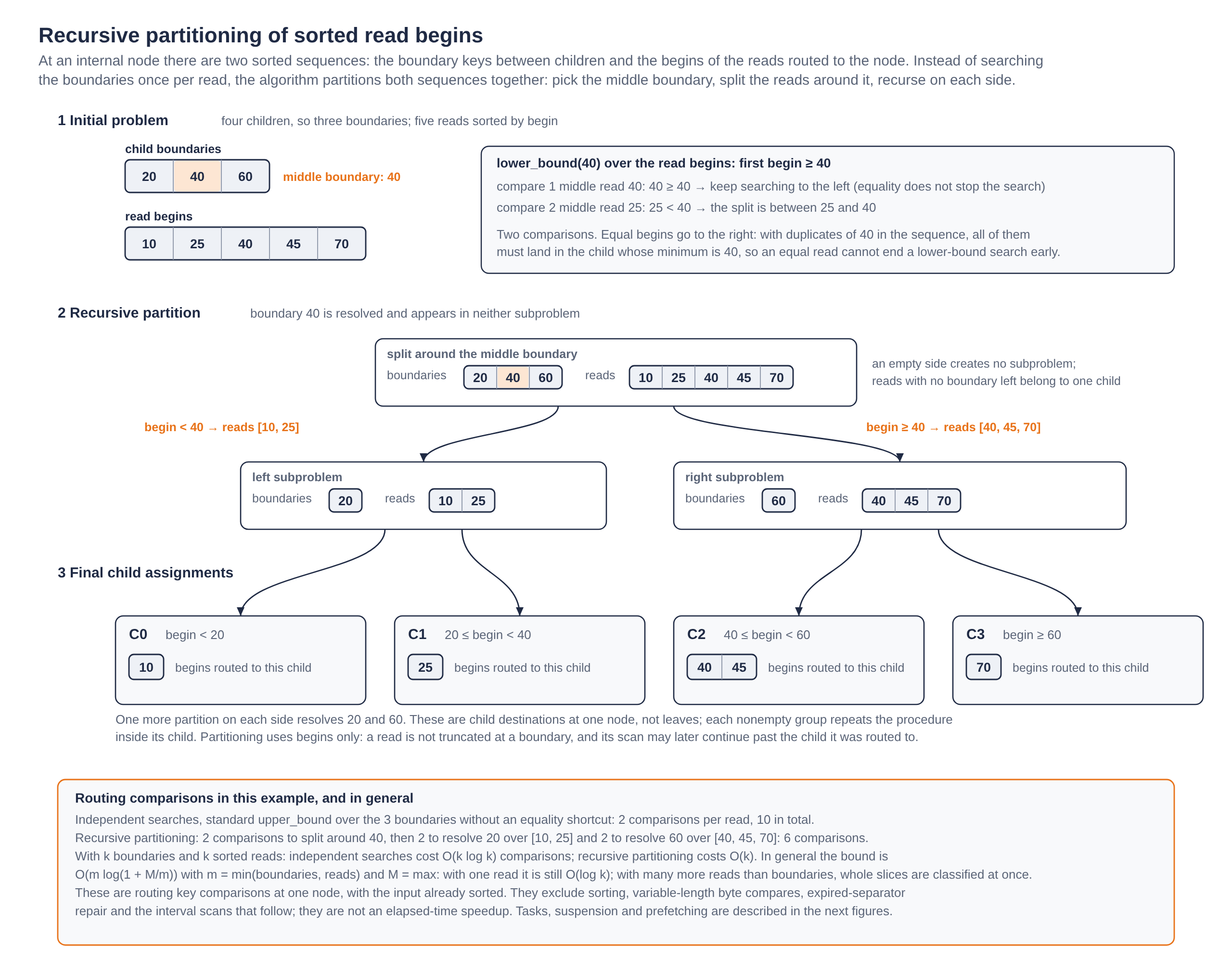
Figure 1. Recursive partitioning of sorted read begins. Boundaries [20, 40, 60] and reads [10, 25, 40, 45, 70]: partitioning around 40 takes two comparisons, and resolving each side takes two more, six in all against ten for independent binary searches without an equality shortcut. Equal begins go right.
How the cost changes down the tree
Let r be the number of reads reaching one internal node and s its number of child boundaries. Independent searches cost O(r log(s + 1)) comparisons. Recursive partitioning changes with the relative sizes of the two sequences:
| Position in a widely distributed batch | Reads and boundaries at one node | Independent searches | Recursive partitioning |
|---|---|---|---|
| Upper levels | Many more reads than boundaries: r ≫ s | O(r log(s + 1)) | O(s log(1 + r/s)) |
| Around the crossover | Comparable numbers: r ≈ s | O(r log r) | O(r) |
| Lower levels | Fewer reads than boundaries: r ≪ s | O(r log(s + 1)) | O(r log(1 + s/r)) |
| A node receiving one read | r = 1 | O(log(s + 1)) | O(log(s + 1)) |
Near the root, a few boundaries route many reads. For a fixed node capacity, independent routing grows linearly with the number of reads, while recursive partitioning grows logarithmically. The upper-level expression can also be written as O(s [log(r + s) − log s]); when r ≫ s, it is approximately O(s [log r − log s]).
Around the crossover, both sequences have comparable sizes. Recursive partitioning takes a linear number of comparisons, while independent searches still perform a logarithmic search for every read.
Near the leaves, the batch has spread among many nodes. The read slices become small, and the advantage diminishes. With one read, recursive partitioning becomes an ordinary binary search over the boundaries. Concentrated reads reach fewer nodes and preserve the opportunity to share comparisons deeper in the tree.
These are costs at one node, excluding input preparation and sorting. The routing cost for the batch is the sum over all visited internal nodes.
A 10,000-read example
A synthetic model in the snapshot uses a tree sized like the 6 GiB campaign’s: a root with two children, four further internal levels with 28 children per node, and 1,229,312 leaves containing 41 history intervals each. It counts comparisons for 10,000 sorted read begins.
For uniformly distributed begins, the changing balance between reads and boundaries is visible level by level. The following table gives an analytical expectation under independent uniform sampling, rather than the counts from one generated batch:
| Level | Nodes at this level | Expected reads per visited node | Independent comparisons, whole level | Grouped comparisons, whole level |
|---|---|---|---|---|
| Root | 1 | 10,000 | 10,000 | 13 |
| Internal level 1 | 2 | 5,000 | 48,571 | 508 |
| Internal level 2 | 56 | 178.6 | 48,571 | 6,993 |
| Internal level 3 | 1,568 | 6.39 | 48,571 | 34,984 |
| Internal level 4 | 43,904 | 1.12 | 48,571 | 47,964 |
| Initial leaf searches | 1,229,312 | 1.004 | 54,634 | 54,414 |
The root has one boundary: independent routing compares it with all 10,000 reads, while the grouped search needs about 13 comparisons. At the next two levels, many reads still share each node’s 27 boundaries. The crossover falls between internal levels 2 and 3. By the last internal level, a visited node receives only about 1.12 reads, so the two methods perform almost the same number of comparisons.
The analytical calculation uses the tree’s geometry and the distribution of reads, without fitting to the generated batch. A subtree covering a fraction p of the history receives a binomially distributed number of reads. For each possible slice size, the calculation averages the binary-search comparison count over the possible split positions, then sums those expectations across the partition tree. Initial leaf searches are counted once per read for independent traversal and once per occupied leaf for grouped traversal. The analytical calculation and its recorded output accompany the sampled model.
The result closely matches the directly counted synthetic batch:
| Comparisons | Analytical expectation | Counted synthetic batch |
|---|---|---|
| Independent internal routing | 204,286 | 204,408 |
| Grouped internal routing | 90,463 | 90,496 |
| Independent routing and initial leaf searches | 258,920 | 259,091 |
| Grouped routing and initial leaf searches | 144,877 | 144,956 |
Both calculations give the same rounded reductions: 56% fewer internal-node routing comparisons and 44% fewer comparisons including the initial leaf searches. The analytical totals differ from the sampled counts by less than 0.1%.
The leaf searches save little in this uniform case: the generated batch reaches 9,959 distinct leaves, almost one per read. Most sharing happens above them. When the same 10,000 reads are clustered within a region of 100,000 history intervals, they reach only 2,400 leaves and share work deeper in the tree. In that counted example, the total falls from 261,795 to 23,643 comparisons, a 91% reduction.
These are comparison counts, not elapsed-time measurements. They cover routing and the initial searches inside destination leaves, with sorted input and live separators. They exclude predecessor checks, overlap scans, cleanup, separator repair, scheduling and the cost of comparing variable-length key bytes. Grouped leaf scans provide further sharing, described below; the evaluation measures the resulting performance.
Grouped reads: shared lookups and fewer repeated comparisons
Partitioning delivers each leaf a slice of sorted reads rather than one read at a time, and the rest of the check is reorganized around that slice.
The in-leaf search happens once per slice: a binary search for the first write at or after the first read’s begin. The predecessor lookup, which v1 repeated for every read, is also shared. The write immediately before that position may extend into the reads, so the task tests that one write against the slice in order and stops at the first read whose begin is at or beyond the write’s end, since every later read begins there too. All these checks reuse the same predecessor.
The forward scan then walks the leaf’s writes in key order against the reads that remain. A read leaves the slice as soon as it is decided: a read that overlaps a newer write is marked as conflicting and dropped; a read that ends at or before the current write’s begin can never overlap a later write and is dropped too. Because read ends are not sorted, a decided read can sit anywhere in the slice, so the unresolved reads are kept as a linked list rather than a contiguous suffix, and each write is compared only against that list. A second cursor remembers the prefix of begins that a write end has already passed; live writes are disjoint and ordered, so those begins are never compared against a write end again.
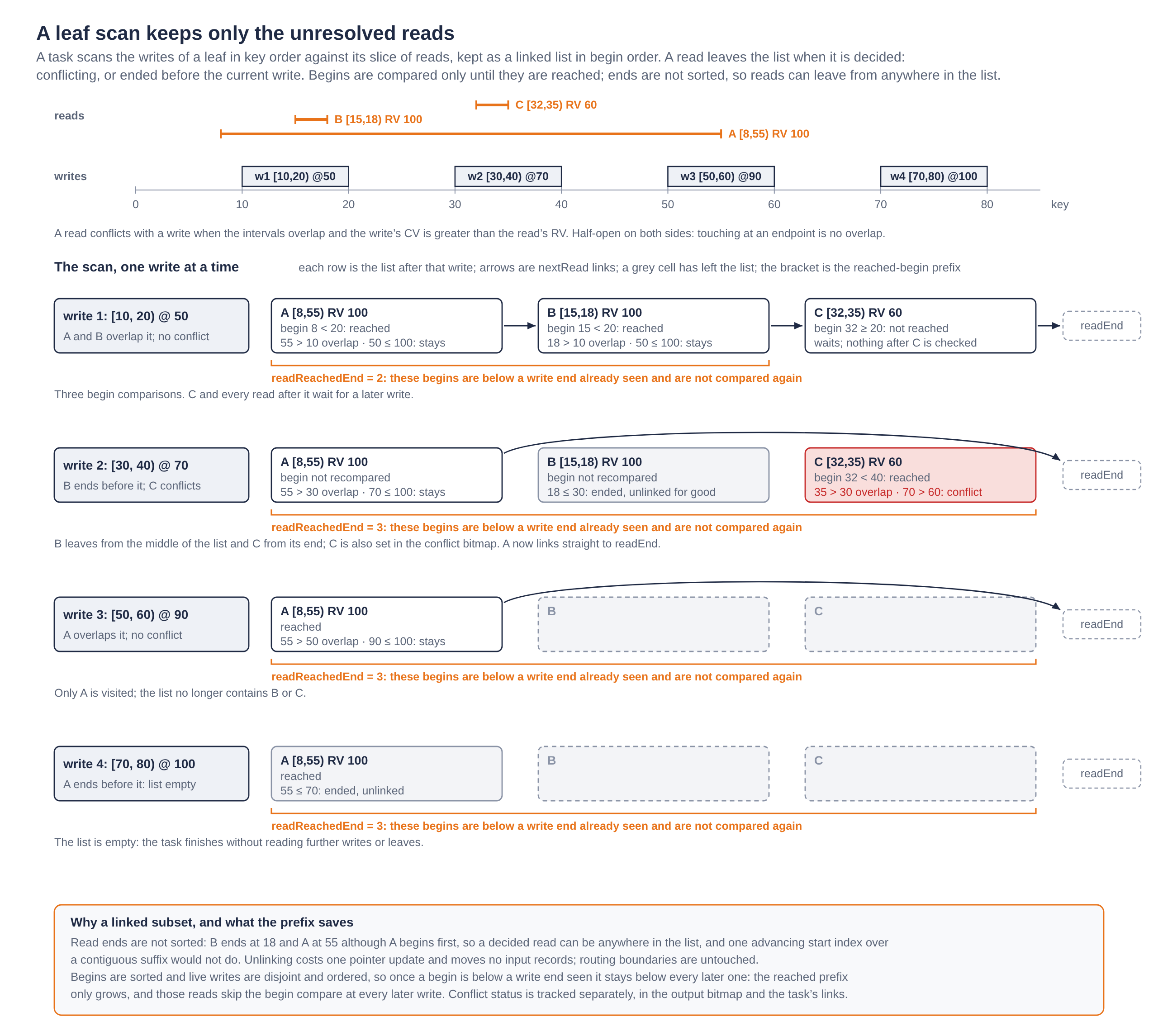
Figure 2. A leaf scan keeps only the unresolved reads. After the second write, B has ended and C has conflicted; only A remains linked. Once a read begin has been reached, later writes do not compare it again.
Each write is checked only against reads that remain unresolved, and begins already reached are not compared again. Long reads that remain unresolved can still be checked against several writes. A read spanning several leaves carries its position across the leaf boundary, where the task prefetches the next leaf before yielding.
Prefetching: distance between a hint and its use
Fewer comparisons reduce the work; prefetching addresses the memory waits between dependent accesses. Separator and leaf keys live in key blocks outside the node, and a descent that fetches them one at a time waits for each. V2 turns every unfinished subproblem into a task: the node it is in, its slice of reads, and the bounds of the search in progress. Up to G tasks (sixteen in the measurements) are resident at once and visited in rounds on a single thread.
A visit does one unit of work: it consumes the memory access the previous visit asked for, advances the task’s state, and before yielding issues a prefetch hint for the access the next visit will need: the next node, the next separator key, the next leaf, the next read begin. While the other resident tasks take their visits, that hint has time to complete. The distance between hint and use is created by the other tasks’ work, which is why interleaving matters even on one thread. When a partition produces two non-empty sides, the task keeps the left one and a new task is created for the right; new tasks join at the end of the round, placed right after the task they split from, so the earliest read ranges stay resident and the suffix is suspended in range order and admitted as slots free up.
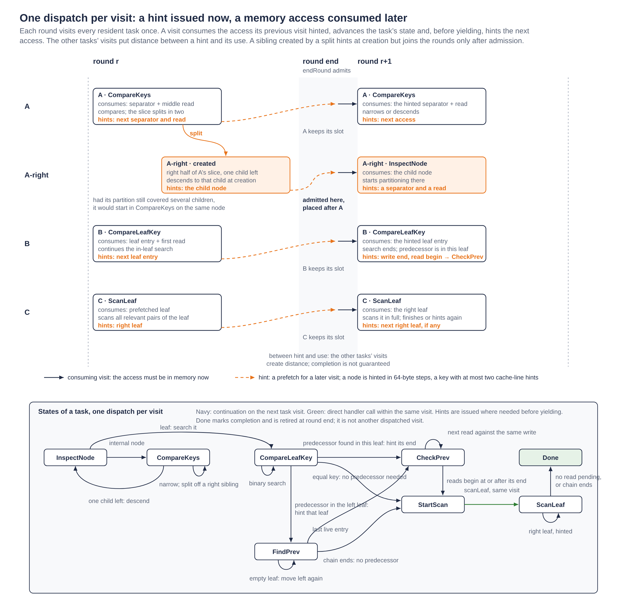
Figure 3. One dispatch per task visit. Dashed arrows are prefetch hints, solid arrows the visit that consumes them; the other tasks' visits create the distance between the two. A hint is a hint: nothing guarantees the line is still cached when the compare runs.
A node is prefetched in 64-byte steps across its full block. A key gets at most two cache-line hints: the line holding its first requested bytes and at most one more. Locating a long key in later blocks can still miss. The granularity of a visit was tuned the other way: earlier versions of v2 scheduled every read–write comparison in a leaf as a separate visit, and profiling showed the dispatch and bookkeeping cost more than the latency it hid. A task now scans a whole leaf in one visit and yields only at the leaf boundary, having hinted the next leaf.
What grouping does to reclamation
V1’s reclamation releases key blocks in allocation order and lets stale references in nodes be cleaned when a search meets them. Grouping adds two hazards.
The first concerns saved positions. Partitioning groups the read begins assigned to each destination leaf, but it does not give a task exclusive ownership of that leaf. A task scanning a long read can enter a leaf that another task reaches by descent; a predecessor search can also enter an earlier leaf. These tasks save positions as ranks, so compacting expired entries after one task has saved a position could invalidate it. Each leaf is therefore compacted on its first visit in a batch, before any task saves a rank, and stamped with the batch number. Later arrivals see the stamp and use the same rank mapping. A leaf left empty stays linked until every task has finished.
The second hazard is the prefetch itself. A separator is a copied reference to a child’s former minimum, and its key block may have been reclaimed and reused while the child still holds live history. V2 checks the separator’s commit version before issuing any key hint; an expired separator is refreshed from the child’s first live entry first, reading versions before bytes. The refresh follows a synchronous descent and can stall, but is paid only when a separator about to be used has expired.
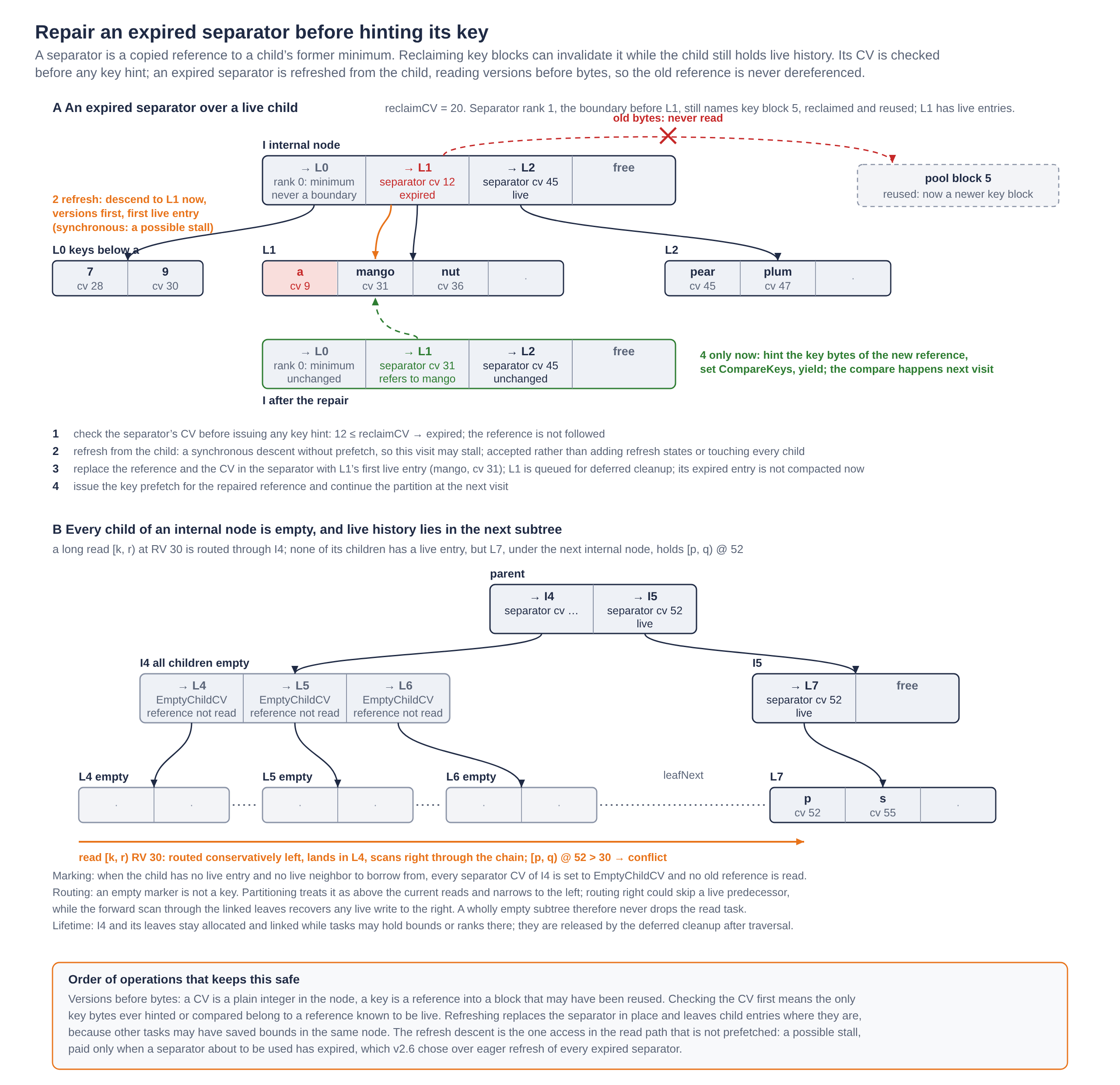
Figure 4. Repair before hinting. Above, the expired separator at rank 1 is refreshed to the child's first live entry and only then prefetched. Below, a node whose children are all empty receives empty-child markers without reading the old separator keys, and a long read routed into it still reaches the live write to its right.
Evaluation testbed
The main measurements come from two Linux machines; an Apple M3 Pro adds a separate standalone comparison. Every timing ratio compares candidates on the same machine and in the same session.
The Linux timing campaigns run one benchmark process at a time, pinned to one core, with no concurrent builds, profiling or other application workloads. V2’s sixteen tasks are interleaved within that single thread.
The Intel machine is an HP OMEN workstation with a Core Ultra 9 285K, a hybrid processor with performance and efficiency cores and no SMT. It has 64 GB of DDR5 RAM, in four 16 GB modules configured at 4,800 MT/s, and runs Linux kernel 7.0.0-38-generic. Timed runs are pinned to CPU 6, a performance core with a 48 KiB L1 data cache, a private 3 MiB L2 and a shared 36 MiB L3. Builds use FoundationDB’s foundationdb/build:rockylinux9-latest container, Clang 19.1.5 and Release configuration; the standalone builds use -O3 -DNDEBUG and libc++. Benchmark output is buffered in memory or written to /dev/shm during timing and copied to disk afterwards. Separate strace checks found no disk writes inside the timed intervals.
A separate random dependent-pointer traversal on CPU 6 measures the latency across the memory hierarchy:
| Working set | Median latency, ns/access |
|---|---|
| Up to 45 KiB | 0.70 |
| 1 MiB | 3.64 |
| 16 MiB | 19.2 |
| 512 MiB | 163.2 |
Each size is warmed up and measured five times, using one dependent pointer per 64-byte cache line and no software prefetch. Measurements use ordinary 4 KiB pages and include address-translation costs; the measurement records include the code, topology and five repetitions per size. The large-working-set latency is about 230× the L1-resident latency, illustrating why the scheduler places useful work between a prefetch and the access that consumes it.
The AMD machine is a Hetzner server with a Ryzen 7 7700, eight cores and sixteen hardware threads, 32 MB of shared L3, one NUMA node and 64 GB of RAM. It runs Linux kernel 6.8.0-138-generic. The controlled campaign of October 30–31 uses CPU 7 and leaves its SMT sibling, CPU 15, idle, launching the container with --cpuset-cpus=7 --cpuset-mems=0. It uses the same build image and Clang version as Intel, with short-benchmark output in memory. Each configuration has one excluded warm-up execution per candidate, followed by three measured rounds with rotating candidate order. All 148 short-benchmark executions, including warm-ups, exit successfully. The campaign records load and dirty memory before each run, CPU and sibling utilization during it, and the full command line.
The Apple M3 Pro contributes a separate standalone comparison, under macOS 27.0.1 with Apple clang 15.0.0 and -O3 -DNDEBUG, with runs interleaved by round and workload.
Both B+ trees use 2 KiB blocks, and v2 uses G=16. Pool sizes depend on the benchmark:
| Benchmark | B+ tree pool or history budget |
|---|---|
| FDB conflictset benchmark | 16,384 × 64 KiB pages: 1 GiB |
| Integrated custom benchmark | 16,384 × 64 KiB pages: 1 GiB |
| Standalone custom benchmark | 1,024 MiB |
| skiplisttest | 262,144 × 64 KiB pages: 16 GiB |
| Long trace | 6 GiB counted-history budget; a pool of 98,300 × 64 KiB pages |
The installed RAM, the tree pool and the counted-history budget are different quantities. Short benchmarks do not fill the tree pools; the long trace exercises capacity-driven reclamation. Its B+ tree runs use ordinary pages, with nr_hugepages=0. History accounting includes the tree’s pool and the additional history storage identified by the harness. Accounting and native timing use separate runs.
Short-benchmark results show three measured rounds and their median. Ratios are calculated within each round before taking the median. Throughput ratios above one are faster; time ratios below one are faster. The measurements cover single-core resolver and component execution.
The full evaluation, Intel manifest and AMD campaign note record the source revisions, binary hashes, parameters and commands.
Workloads
Four workloads exercise different parts of the resolver. The custom workload runs both through FoundationDB and directly against the trees, giving five execution paths in total.
FoundationDB’s conflictset benchmark measures complete batch resolution. Each transaction has four read-conflict ranges and two write-conflict ranges over a ten-million-key space. The point workload accesses individual keys; the range workload uses reads spanning 1–1,000 keys and writes spanning 1–10. Each execution has 1,000 warm-up batches followed by 2,000 measured batches of 500 transactions: one million measured transactions. This workload includes transaction-level rejection and intra-batch conflicts, rather than timing independent read checks alone.
FoundationDB’s skiplisttest separates read checking, write merging and the overall conflict-detection interval. The campaign uses 500 batches of 40,000 ranges, span 10 and seed 1. Seven key configurations vary length from 16 to 128 bytes and place the distinguishing bytes before a common suffix or after a common prefix. This exposes the cost of locating and comparing key bytes as well as traversing the index.
The custom point/range workload separates historical read checking from write application. With seed 1234, each batch generates 4,000 reads and up to 1,000 sorted, disjoint writes over ten million logical keys, encoded as 12-byte keys. In the range workload, lengths are drawn from 1–20 keys, with one in ten draws using 1–2,000 instead. Read versions lag the batch’s commit version by up to 500 version units. Each execution processes 3,000 batches and twelve million reads.
The integrated version, named macBenchmark in the harness, submits this workload through FoundationDB’s resolver batch path and can compare all three histories. Each read is a separate transaction; the writes form a final read-free transaction. The standalone version calls the B+ trees directly and excludes FDB’s skip list. Input generation is outside the timers; v2’s endpoint preparation and sorting are also outside the standalone read timer. Its rates therefore describe checking prepared inputs. Reported integrated totals are sums of instrumented phases, not whole-process wall time.
The long trace tests retention and reclamation under a fixed memory budget. It replays a 5,400-second segment of pilot-2000M-l0-7200.trace: 172,800 batches, each representing 31.25 ms and containing 2,048 transactions. Both trees start from the same cold segment boundary and receive the same offered work under a 6 GiB counted-history budget. Retention and decision comparisons use accounting runs; Intel additionally has three native v2 timing runs. Archived v1 and FDB accounting records are used for retention and memory, without turning their different sessions into a timing comparison.
What the measurements say
V2 substantially improves read checking over v1 in the custom workload and skiplisttest. Its position against FoundationDB depends on the workload: range reads are faster in the integrated custom benchmark, while point reads remain slower. Write application remains expensive, and the complete-batch results include a regression on conflictset ranges.
Read checking and write application
In the Intel standalone benchmark, the sequential fork-v1 tree and v2 use one common harness. V2 reaches 2.11× v1’s point-read throughput and 1.46× its range-read throughput. Write throughput is 0.88× and 0.91× v1’s, respectively. These measurements cover the changes between the two implementations; they do not separately attribute the gain to partitioning, grouped scans or prefetching.
Through FoundationDB’s resolver batch path, the Intel custom workload gives v2 0.90× FDB’s point-read rate and 1.14× its range-read rate. Its write rates are 0.52× and 0.65× FDB’s.
The controlled AMD campaign has the same direction with different magnitudes. In the integrated custom workload, v2’s read check takes about 0.49× v1’s time on points and 0.63× on ranges. Against FDB, it takes about 1.40× on points and 0.955× on ranges. Including the other instrumented phases, v2 takes 0.62× and 0.71× v1’s time, but 1.55× and 1.07× FDB’s. In the AMD standalone comparison, read-check times are 0.647× and 0.759× v1’s.
The separate Apple M3 standalone session gives 2.23× and 1.50× its v1 baseline’s read throughput. Its different baseline and less controlled execution conditions prevent treating those ratios as another sample of the Intel or AMD comparison.
FoundationDB’s benchmarks
In the Intel conflictset benchmark, v2’s complete-batch throughput reaches 0.89× FDB on points and 0.97× on ranges. V1 reaches 0.64× and 1.08×, respectively.
The controlled AMD campaign exposes a larger range-workload regression. V2 takes 1.298× FDB’s batch time on points and 1.194× on ranges. Against v1, its ratios are 0.746× on points but 1.244× on ranges: v2 improves points and makes ranges slower. The range read check itself rises from 1.377 seconds in v1 to 1.829 seconds in v2, compared with FDB’s 1.469 seconds. Grouping therefore does not improve every read workload.
In skiplisttest, v2 reduces read time consistently across the seven key layouts, but write merging offsets the savings against FDB.
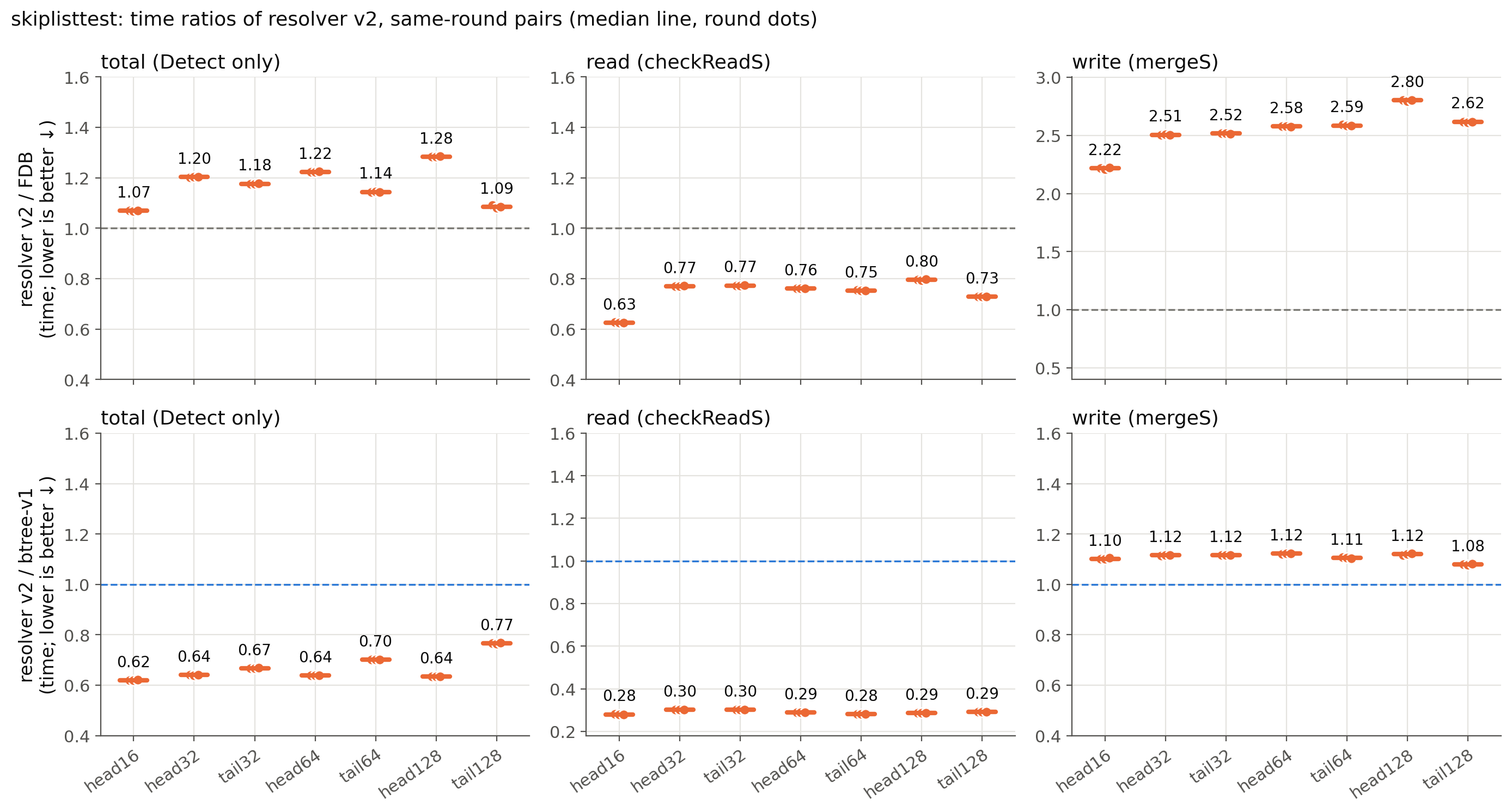
Figure 5. FoundationDB's skiplisttest on Intel, seven key layouts, time relative to FDB and to v1. Reads take 20–37% less time than FDB's skip list; write merging takes 2.22–2.80× as much; total conflict-detection time is 1.07–1.28× FDB's. Lower is better.
On AMD, skiplisttest gives v2 0.81–0.96× FDB’s read-check time, 2.30–2.60× its write-merge time, and 1.15–1.34× its total time. Against v1, total time falls to 0.69–0.80×, a 20–31% reduction in execution time.
Retention and the remaining cost
Retention is effectively unchanged. On the long trace, both trees first discard history about 702.9 seconds into the segment and finish with a minimum retained age of 582.9 seconds under the same 6 GiB budget. Their curves nearly overlap, with matching offered and decision hashes and no rejections for age or memory.
FDB’s 265-second window was calibrated against the same 6 GiB history budget by replaying the trace with different fixed windows and measuring peak live skip-list memory. A 265-second window peaked at 5.92 GiB, using 98.64% of the budget; 270 seconds exceeded the budget after 2,199 seconds of trace time. We therefore use 265 seconds, the largest tested window that fits, as the reference. Under that budget, both B+ tree versions retain at least 582.9 seconds over the measured post-discard interval: 2.20× as much history. The v1 evaluation records the calibration.
Over the final 600 seconds of trace time, the B+ tree’s retention falls by 0.62% (3.66 seconds), while FDB keeps its 265-second window and its counted history memory increases by 0.0035% (0.222 MB). These are the observed changes over that interval, calculated from its endpoints in the per-batch records.
Intel’s native timing runs show where v2 spends the remaining time.
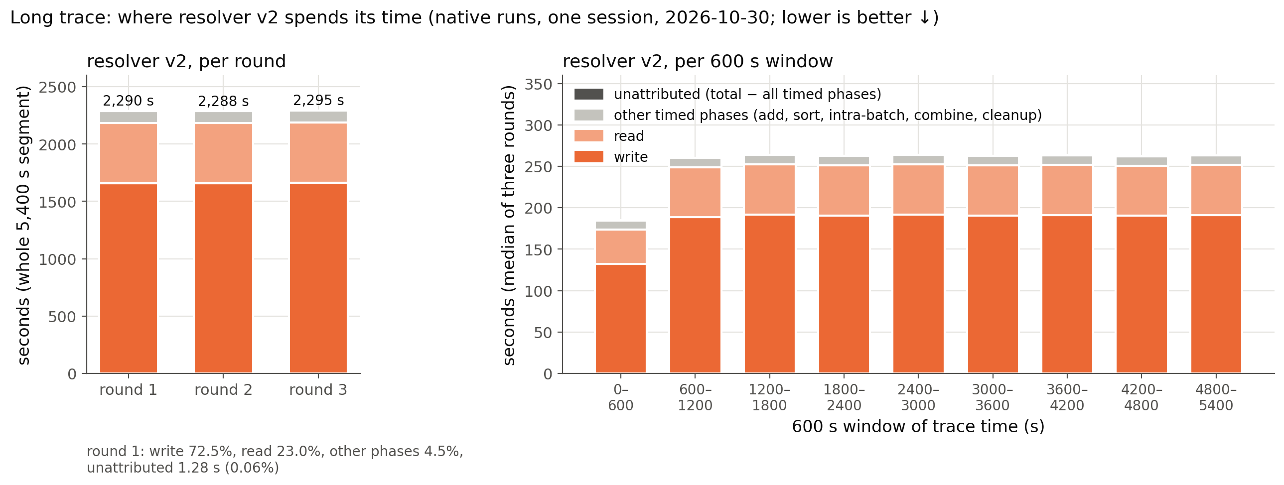
Figure 6. Native v2 time on the long trace. In the first round, writes account for 72.5%, reads for 23.0% and the other timed phases for about 4.5%; approximately 0.06% is unattributed. Writes remain sequential, applied one interval at a time.
V2 preserves v1’s retention while reducing read costs in several workloads. Sequential write application now dominates the long-trace runtime, although the conflictset range regression also remains to be explained.
All these measurements predate the public branch’s write-reservation fix. For the key lengths in these workloads, the corrected code retains the same 35-block reservation, and separate validation finds the same decisions. The added computation per write has not been timed, so these remain measurements of the recorded revisions, rather than of the corrected public head.
Search of similar approaches
Once the partitioning was working and the comparison counts came out as they did, it looked too good, and the problem it solves is too general, for nobody to have met it before: a sorted sequence of keys to be located in another sorted sequence is one of the oldest problems in the book. So I did an AI-assisted search of the literature to see what was already there. The answer is that the mechanism is classical, and the names are worth having.
For sequences of sizes r and s, let m = min(r, s) and M = max(r, s). The comparison bound O(m log(1 + M/m)) belongs to the classical merging literature: Hwang and Lin (1972) give a comparison-efficient merging algorithm, and Brown and Tarjan (1979) give an asymptotically optimal merging algorithm for tree-represented lists. Splitting one sequence around a pivot, binary-searching the other and recursing on the two sides is also the pattern used by parallel merge. CLRS presents it as P-MERGE, choosing the pivot from the longer input; this traversal always chooses a child boundary. Over a tree, sharing the search of a sorted batch belongs to the family of multisearch algorithms, with Arge’s buffer trees (1995) as an external-memory relative.
In databases, Zhou and Ross (VLDB 2003) buffer index lookups per node to improve cache behavior, including workloads with interleaved updates. FAST (Kim et al., SIGMOD 2010) combines blocking by page, cache line and SIMD width with pipelined searches, and uses order-preserving partial keys to handle longer keys. PALM (Sewall et al., VLDB 2011) extends batch processing to B+ tree queries and modifications.
On the prefetching side, Chen, Gibbons and Mowry (SIGMOD 2001) model the latency and overlap of cache-line transfers to choose node width and scan lookahead. Asynchronous memory access chaining (Kocberber et al., VLDB 2015) keeps independent lookup states so that irregular traversals can progress separately. Psaropoulos et al. (VLDB 2017) express interleaving with coroutines and model how computation and switching overhead cover memory latency; Jonathan et al. (VLDB 2018) examine the technique across several pointer-based structures.
The comparison model in this post instantiates the routing algorithms on a concrete synthetic tree: counts per level, the initial leaf search included, and uniform and clustered reads considered separately. It counts the comparisons performed by the two algorithms; it does not turn an asymptotic bound directly into an execution-time estimate. The analytical expectation then averages those comparison counts over the declared read distribution. Extending this to cache-line accesses, reuse and prefetch distance would connect it to the systems models above and help predict G. That extension should use the same workload as the timing experiment: the 44% comparison reduction belongs to the 10,000-read, 6 GiB example, while the 2.1× throughput result comes from the standalone benchmark.
For this resolver, making those techniques fit requires temporal routing and lifetime rules: half-open ranges, equal begins routed right, empty-child markers routed conservatively left, and predecessor checks shared by a slice. A batch can encounter references invalidated by earlier reclamation, and interleaved tasks can save positions in the same leaf. V2 refreshes expired separators before hinting their keys, compacts each leaf before any task saves a rank, and defers structural removal until all tasks finish. Those are the implementation choices developed in the design document.
A pity I did not run the search before reinventing the mechanism; it would have saved me a week of work. Still, I am happy to have invented something relevant, even decades after it was invented for the first time.
What comes next
The read path did what it was built to do, and in doing so it moved the bottleneck. Writes account for nearly three quarters of the time on the long trace and outweigh the read savings against the skip list in skiplisttest. Each write interval still takes its own descent, so writes are the next target for sharing search work and overlapping memory accesses. The next milestone routes a batch’s writes the way v2 routes its reads: one partitioned descent for a mixed sequence of read and write begins, writes applied after acceptance at destinations recorded during the descent. That changes who owns a leaf while a batch is in flight, so it needs its own design and validation. After the resolver, the series moves to the storage server.
Milestone record
The milestone record brings together the implemented design, evaluation and supporting records. It identifies the measured revisions separately from later code changes.
The design as implemented describes partitioning, tasks, scheduling, the leaf scan and the safety rules, with twelve figures. The decision record follows the versions from v2 to v2.6; the journal records when things happened. The evaluation has every table and figure for Intel, AMD and Apple M3 with the scope of each, and the evidence register ties the claims to source identities, tests and replays. The engineering overview is the five-minute version, and the project architecture places the resolver in the retention protocol. The 10,000-read comparison counts come from a small model with its recorded output, kept under analysis/ alongside the analytical expectation and the final-interval retention and memory calculation. The code, tests and benchmarks are on the resolver-v2 branch of the FoundationDB fork, and the measurement records that do not fit in the repository are assets of the release resolver-v2-evaluation.